Four decades of questions from the FTD community, answered — from how automated counting really works to what to do about dust in your microscope.
Since 1979 our equipment has automated complex, tedious processes — but it has never pretended to replace the expert. In FTD that journey ran from automatic sample positioning with manual "clicker" counting, through drawing tubes and digitiser tablets, to on-screen counting, and now to fully automatic capture and counting.
Our systems do not make the final scientific decisions: they do not decide what is or is not a fission track, or exactly where a track ends. What they do is eliminate the fatigue of repetitive work and present the expert with a small, high-quality candidate set instead of an enormous raw one. Every entity the system recognises is documented in a data table, and our latest software stores a complete three-dimensional image stack of each grain, so you can always return to the source data.
The automatic counting systems genuinely run without operator intervention during capture and counting. There is an initial set-up per sample and a final review-and-edit pass — for example, overlapping track clusters that even a human struggles to separate are estimated by the software but can always be overridden by the operator.
Two advantages deserve emphasis: automation counts densities well beyond what a human can conveniently manage, and — unlike a human, whose counts vary with fatigue, interest and eyesight — the machine is perfectly consistent under identical conditions. Results from a substantial number of installations have borne this out.
Fission tracks in apatite are counted automatically by capturing both reflected- and transmitted-light images and using them to discriminate genuine tracks from non-track objects. The uranium content of the apatite is measured by laser-ablation ICP-MS, which avoids the time-consuming irradiation step of the external detector method.
If you prefer to continue with the external detector method, the same module automatically counts the induced tracks on the mica detector as well.
The software is split into two packages — TrackWorks, which creates the data files and images at the microscope, and FastTracks, which lets the analysis be carried out anywhere in the world using those files. Within them, the process has three stages:
The countable track density limit is roughly an order of magnitude higher than for manual counting, and review takes a fraction of the time of a manual count — with far greater consistency.
Yes, you can. One reason the new LA-ICP-MS workflow was developed is that it bypasses neutron irradiation — access to suitable reactors is becoming difficult in some countries. But we are equally aware that some laboratories have no convenient access to an LA-ICP-MS instrument.
The software therefore supports both techniques. In fact, automatically counting tracks on the mica detector — with its clean background — is considerably easier than on the apatite grain with its many artefacts.
Estimates supplied by workers in the discipline, for a typical sample of 20–30 grains:
The automatic capture and counting steps are fast — it is the remaining manual steps that dominate. For comparison, counting a sample entirely by hand takes around three hours of intense, error-prone labour, and is simply impossible at the higher track densities the automated system handles comfortably.
Several calibration steps are needed, but each only once. The essential tool — supplied with every full Autoscan system — is a stage micrometer: a slide engraved with very accurately positioned fine lines.
The optical train must be calibrated for each objective/Optovar/camera/C-mount combination in use. The procedure, built into our software, involves placing the stage micrometer under the microscope and entering the number of microns visible across the screen horizontally and vertically. This creates a microns-per-pixel constant for that combination, so any distance clicked on screen converts immediately into real microns. It is carried out for each objective at installation.
Recalibration is only needed when an element changes — different objective models have slightly different magnifications, cameras different pixel sizes, C-mounts different lens factors. One caution: total magnifications beyond 1000× produce only "empty magnification". The Rayleigh resolution limit has already been reached; the image gets bigger and blurrier, adding no information — however much psychological comfort it may offer.
We have not yet developed a fully automated module for confined track lengths — that is our next objective, and a further research project with Prof. Gleadow's group is planned. Existing clients will be offered a software upgrade path once it is achieved.
In the meantime, our systems measure track lengths semi-automatically: the high-resolution camera presents a high-quality image on screen, and the operator clicks each end of the track. The measurements are highly accurate; they simply still involve a human.
Oil occurs where suitable prehistoric organic matter was buried in rock that then experienced the right thermal history to turn that matter into oil. Assessing a prospect therefore requires knowing the age of the rock and its temperature history — and fission track dating provides both, using marker minerals such as apatite, zircon and sphene that contain traces of natural uranium.
As uranium atoms fission over geological time, they leave microscopic damage tracks in the crystal. Counting the accumulated tracks reveals age (in the external detector method, by comparison with tracks induced in a mica detector at a research reactor — in Australia, ANSTO's OPAL facility). Because heat "anneals" and shortens tracks, the statistical distribution of track lengths reveals the time-temperature history.
The observational challenge is severe: tracks are under 16 µm long and about 1 µm across — close to the resolution limit of visible light — and at the 1000× magnification required, the whole track is never in focus at once. That is why high-quality 3-D imaging is essential to the analysis.
With offshore drilling costing on the order of a million US dollars a day, telling someone to drill in the wrong place does nothing for one's popularity. Core samples are still taken — the analysis is simply of far higher quality.
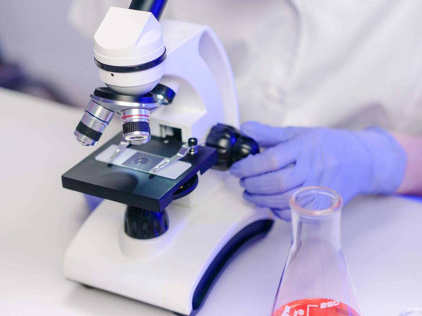
It happens in the best of families. After the panic subsides, the task is to work out where the dust is. These notes refer to our typical Zeiss-based systems, but apply broadly.
Start with the camera — the easiest check. Rotate the camera: if the spots stay put, the dust is on the camera chip. Remove the camera and very carefully blow the dust off. Never rub the fragile sensor, and avoid paper tissues — they contain clay, are abrasive, and drop lint. Use a proper lens cloth, a blower brush (never touch the bristles — skin oils transfer to everything you clean) or canned air. For solvents, isopropyl alcohol is best as it leaves no residue; pre-impregnated wipes are excellent. Avoid harsh solvents such as turpentine or petroleum — in severe cases they attack lens cements and plastic finishes.
If the spots move when the camera rotates, work your way down the optical path: